Odds Favour A bottom For Silver


 Introduction
Recent explorations of the phenomenon of preferred gradients have revealed two very important facts about the interaction between price and preferred gradients.
The first is that charts of longer duration serve much better to perform accurate analysis, largely because they are relative fewer dense clusters of small trend reversals that make it difficult to find the correct locations for the trend lines.
Secondly, while the channel ratios of channel pairs (i.e. the combination of three parallel trend lines) plays an important role in deciding where to locate trend lines that represent preferred gradients. Some ratios are particularly important; of these the most important are the 500:500 ratio, showing the channel pair is divided into two equal parts; the 382:618 Fibonacci ratio and the 400:600 ratio.
Other ratios rise in importance when there are two or more channel pairs with that same ratio.
A recent focus on monthly closing prices has shown some amazing results. Silver is one of these to demonstrate that the phenomenon displays very high accuracy over many decades even when monthly prices are analysed.
Silver monthly closing charts
The first chart uses only three trend lines to present clear evidence of the existence of this phenomenon. Briefly, key features of preferred gradients include:
- Prices tend to change or reverse trend along preferred gradients
- One can identify many different preferred gradients on a price chart
- Parallel occurrences of the same preferred gradient – as channel pairs – tend to hold to the better known channel ratios, or repeat the same channel ratio
- Different preferred gradients on a chart differ according to the Fibonacci ratio
When doing an analysis, the procedure is always to begin with one trend line drawn between two significant reversals. This is the master line and all other trend lines in the analysis have gradients that are derived from the master gradient. Experience has shown that doing so results in a more credible analysis.
Like the gold price, the silver price is heavily manipulated, at least during the past decade and more. The nature of the analyses below show that there are forces at work in market prices that – in the case of silver – are greater than the effects of the manipulation. This is not to say that manipulation does not bring results, but that when the price is manipulated, the end results is still determined by whatever it is that is responsible for this phenomenon.
The new price might be much lower or higher than what it might have been if there had been no manipulation, but the actual and manipulated price still fits the overall structure or pattern defined by the phenomenon.

Chart 1. Silver Monthly close. Last = $14.08
In Chart 1, the master line M is generated between the lows of the deep ‘V” tops of the highs in 1980 and in 2011. Experience has shown that such formations, known as ‘bifurcated tops’ – also bifurcated lows – develop around a significant preferred gradient so that the low of the ‘V’ lies right on that gradient.
That this is true of the silver monthly chart is confirmed by line P, which is drawn exactly parallel to line M, from the peak of the 1980 bull market. Line P passes by the outright 2011 top with an accuracy of 0.09%, expressed relative to the vertical scale of this chart ($1.307 to $48.70). This is very accurate, seeing that the two peaks are 31 years apart. The actual difference is 4.3 cents.
Line F, also generated from the 1980 top, illustrates the effect of changing a master gradient by the Fibonacci ratio. The gradient of line F is shallower than that of line M by 0.618034, the Fibonacci ratio. It is clear that line F ‘somehow’ passes close to the bottom of the second ‘V’ low after the 2011 top. Line F miss the actual low by 1.1 cent for a difference of 0.04%, doing even better than line A. The probability that this is the result of coincidence must be vanishingly small.

Chart 2. Silver Monthly close. Last = $14.08
Chart 2 uses the same master line, M, as was used in Chart 1. The analysis shows four channel pairs:
- VMW with line M as the centre line and line and line V the same as line P in Chart 1. With lines V and M fixed in unique positions, line W was located so that the channel ratio of VMW is exactly 400:600, one of the important ratios
- ABC has line B so located that it passes through the 2011 top. Lines A and C are drawn tangent to the whole chart; these three uniquely positioned trend lines have a channel ratio of 497:503, just marginally away from a 500:500 ratio of a channel that is evenly divided
- XYZ has lines X and Z at significant reversals, a low and a top, while line Y is so located that the channel ratio is 499:501, even closer to being evenly divided than channel ABC
- PQR, which also fits the chart very well indeed, has a 400:600 ratio, exactly the same as channel VMW
Careful examination of the different channels will show that at least two lines of the three are located in unique points, which argue against ‘engineering’ of the analysis in order to achieve the desired results. The fact that there are reversals, even small ones as in the case of line W, that enable the ratios as recorded, supports the view that prices reverse trend at preferred gradients and that these display channel ratios that conform across many analyses.
Interpretation
Readers may have noticed that a line of three of the channel pairs pas very close to where the price of silver was recently fixed. The monthly closing fix for November, December and January are: 14.08, 13.82 and 14.08. The trend Table in the upper left corner shows the values of these lines for the February close. It is evident that line W is acting as support, while the other lines set a challenge for silver during the coming months. Lines C and Y set a mild challenge, while line Q requires a good run in the price to be tested.
At the end of 2015, with the fix on 31 December at $13.82, the value of line W was $13.832, for a difference of 0.025%. It would seem there is a reasonable prospect that this could be the low monthly close of the almost 5 year bear market in silver. However, confirmation has to come soon – February or March – with a clean break above the resistance offered by lines Y and C to hopefully confirm a new trend.
Readers who noticed the projected value for line C is higher than the closing price for silver, should not be concerned. Line C is drawn from the December close and at the end of January it is still below the price. The price has to gain at least to $14.15 by the end of February to remain above line C and recover above line Y after a very minor break below the blue line.
Conclusions
Analyses of monthly closing values present clear evidence that preferred gradients do exist and that they present with specific channel ratios as a key feature. Further, they do so with high all-round accuracy over a time span of many decades – from 1968 to 2015 in this instance, a time span of 47 years. The structure is maintained accurately as the price accommodates to the effects of manipulation and constant intervention since 2011 in particular.
The structures on these two charts completely demolishes the accepted hypothesis that price history cannot be used to anticipate the future behaviour of the price.
Finally, credible – yet never absolute – evidence is that silver has bottomed.
©2016 daan joubert, Rights Reserved
chartsym (at) gmail(dot)com
More from Silver Phoenix 500